
Episode 3: Part 2 of the 1996 Presidential Elections
Introduction
At the end of Part 1 of Episode 3 on my series on Ghanaian elections, I performed a quick sum of the percentage values obtained by the political parties grouping them by region and some had 101%. This figure was exclusive of the percentage of rejected ballots.
Sum of Percentage Values Per Region for Parties
This did not sit well with me, so I decided to enquire from people whom I believe know much about elections than myself.I learnt that the percentage vote for each party is calculated as:
(Number of Party's Votes/**Total Number of Votes**)*100%.
This was right by me as the sum of all percentage values for each party and the percent of rejected ballots grouped by region should add up to 100%. But I realized the percentage values from the original dataset was calculated as:
(Number of Party's Votes/**Total Number of Valid Votes**)*100%
Hence the difference in both calculations is the denominator.
NB:
So I got my Disqus up and running. Please let me know what you think about the method of calculating the percentage values for each political party. Come on let us discuss!! (no pun intended)
With this idea in mind, I will have to update the final dataset from Episode 3. Join me on this journey of data updating
Importing Library and Reading In Data
library(tidyverse)

vote_data <- read_csv("votes_data_1996.csv")
vote_data <- vote_data[, -1]
head(vote_data)
## # A tibble: 6 x 12
## Region `J.J Rawlings` `NDC%Vote` `J.A Kufuor` `NPP%Vote` `E.N Mahama`
## <chr> <dbl> <dbl> <dbl> <dbl> <dbl>
## 1 WESTE~ 405992 57.3 289730 40.9 12862
## 2 CENTR~ 330841 55.2 259555 43.3 8715
## 3 GT AC~ 658626 54.0 528484 43.3 32723
## 4 VOLTA~ 690421 94.5 34538 4.73 5292
## 5 EASTE~ 459092 53.8 384597 45.0 10251
## 6 ASHAN~ 412474 32.8 827804 43.8 17736
## # ... with 6 more variables: `PNC%Vote` <dbl>, Valid_Votes <dbl>,
## # Rejected_Ballots <dbl>, Tt_Votes_Cast <dbl>, Tt_Reg_Voters <dbl>,
## # `Turnout%` <dbl>So I will be using my favorite R library tidyverse only as it contains all the functions I will need. Next, I am going to read in the data, it is available for download here. This is a cleaned up but not final version of the data downloaded from the Electoral Commission of Ghana’s website. Below are a few actions I performed on it
- Removed few rows.
- Renamed the columns.
- Removed all row and sum totals.
And if you would like to know the details on the above steps,check the sections from Importing Libraries and Data Extraction to More data cleaning in Episode 3 of the blog series. In the final line of the code above, first column which is an auto-increment value from 1.
Structure of the dataset
dim(vote_data)## [1] 10 12summary(vote_data)## Region J.J Rawlings NDC%Vote J.A Kufuor
## Length:10 Min. :145812 Min. :32.79 Min. : 21871
## Class :character 1st Qu.:340638 1st Qu.:54.30 1st Qu.: 93481
## Mode :character Median :400687 Median :59.21 Median :245006
## Mean :409946 Mean :61.41 Mean :283488
## 3rd Qu.:447438 3rd Qu.:67.18 3rd Qu.:360880
## Max. :690421 Max. :94.55 Max. :827804
## NPP%Vote E.N Mahama PNC%Vote Valid_Votes
## Min. : 4.73 Min. : 5292 Min. : 0.7247 Min. : 195437
## 1st Qu.:21.26 1st Qu.:10904 1st Qu.: 1.4210 1st Qu.: 600659
## Median :38.44 Median :16186 Median : 2.0501 Median : 674529
## Mean :31.86 Mean :21114 Mean : 4.5293 Mean : 714547
## 3rd Qu.:43.32 3rd Qu.:31481 3rd Qu.: 5.0658 3rd Qu.: 823018
## Max. :45.04 Max. :45696 Max. :14.2010 Max. :1258014
## Rejected_Ballots Tt_Votes_Cast Tt_Reg_Voters Turnout%
## Min. : 0 Min. : 206200 Min. : 272015 Min. : 0.00
## 1st Qu.: 4518 1st Qu.: 615029 1st Qu.: 783210 1st Qu.:72.59
## Median :10384 Median : 685494 Median : 900378 Median :78.76
## Mean : 9327 Mean : 725658 Mean : 927961 Mean :62.72
## 3rd Qu.:12024 3rd Qu.: 825604 3rd Qu.:1034002 3rd Qu.:80.41
## Max. :22387 Max. :1270071 Max. :1592854 Max. :81.84Have you noticed some columns have 0 as a value, let me give you a clue. Check the minimum values. Time is up, the image below shows the columns which have this value.
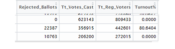
Columns with 0
- Number of Rejected Ballots for the NORTHERN REGION.
- % turnout for the NORTHERN REGION.
- % turnout for the UPPER WEST REGION.
Fortunately, these are values can be calculated in a few steps:
- For 1: Subtract the number of valid votes from total registered votes.
- For 2 & 3: Calculate the Turnout percent for points 2 and 3
These calculations will be done along the line.
Storing Non-Percentage Columns
non_percent <- vote_data[, !grepl("%", colnames(vote_data))]
colnames(non_percent)
## [1] "Region" "J.J Rawlings" "J.A Kufuor"
## [4] "E.N Mahama" "Valid_Votes" "Rejected_Ballots"
## [7] "Tt_Votes_Cast" "Tt_Reg_Voters"head(non_percent, 2)## # A tibble: 2 x 8
## Region `J.J Rawlings` `J.A Kufuor` `E.N Mahama` Valid_Votes
## <chr> <dbl> <dbl> <dbl> <dbl>
## 1 WESTE~ 405992 289730 12862 708584
## 2 CENTR~ 330841 259555 8715 599111
## # ... with 3 more variables: Rejected_Ballots <dbl>, Tt_Votes_Cast <dbl>,
## # Tt_Reg_Voters <dbl>Next, a dataframe of columns whose values are not percentages: that are of the integer data type are separated since the rest of the calculation is based on them. In creating the dataframe, I used regular expressions to extract all columns without the % sign in its name.
Creating the calc_percent function and Calling it
calc_percent <- function(col1, col2){
    return ((col1/col2) * 100)
}
Using the formula stated in Introduction, the function calc_percent is created. The details for the function are as follows:
- The function takes 2 arguments:
- col1: column whose percentage value we are interested in. Example: % of NDC’s votes in the Northern Region
- col2: column that has the total value. Example: Total Number of Votes in the Northern Region.
- col1 is divided by col2 and the result is multiplied by 100% to return the percentage value of col1.
- The result above is returned to the variable that called the function.
- Also, note that the result of this function will be a Series of percentage value for each of the 10 regions.
Moving on, I called this function to calculate the percentage of turnout for each region, the result was stored under the name Percent_Turnout and assigned back to the non_percent dataframe.
non_percent["Percent_Turnout"] <- calc_percent(non_percent$Tt_Votes_Cast,non_percent$Tt_Reg_Voters)

non_percent[, c("Region", "Percent_Turnout")]
## # A tibble: 10 x 2
## Region Percent_Turnout
## <chr> <dbl>
## 1 WESTERN REGION 74.5
## 2 CENTRAL REGION 79.1
## 3 GT ACCRA REGION 78.4
## 4 VOLTA REGION 81.8
## 5 EASTERN REGION 81.1
## 6 ASHANTI REGION 79.7
## 7 BRONG AHAFO REGION 72.0
## 8 NORTHERN REGION 77.0
## 9 UPPER EAST REGION 80.6
## 10 UPPER WEST REGION 75.8The output shows usually more than 2/3rds of the registered voters come out to vote for the presidential elections.
Rightaway, I question I am interested in answering after the data extraction for all the Ghanaian elections will be How much have this value changed since the 1992 elections till 2016 elections?
Remember, the 0 values?
Fortunately, 2 & 3: the Northern and Upper West Region have values for the column Turnout%. The lone ranger now is 1: Number of Rejected Ballots in the Northern Region. For this value only, I will re-calculate the number of rejected votes. This can be found in the column Rejected_Ballots.
The formula is: Rejected_Ballots = Tt_Votes_Cast - Valid_Votes
# number of rejected votes
non_percent["Rejected_Ballots"] <- non_percent$Tt_Votes_Cast - non_percent$Valid_Votes

# confirm Northern Region now has a value
non_percent[8, c("Region","Rejected_Ballots")]
## # A tibble: 1 x 2
## Region Rejected_Ballots
## <chr> <dbl>
## 1 NORTHERN REGION 17840About 17,000 of rejected ballots, this is a huge figure. TO put this into perspective, in 2016, the only Independent candidate; Jacob Osei Yeboah pulled 15,889 votes from all the regions.
Going back to the function calc_percent, it is used to find percentage values per region for the details below. All of these would be assigned back to the non_percent dataframe as columns
- Valid Votes
- Rejected Votes
- Votes for NDC party
- Votes for NPP
- Votes for PNC
# confirm the number of columns before calculation
dim(non_percent)
## [1] 10 9# percentage of valid votes
non_percent["Percent_Valid_Votes"] <- calc_percent(non_percent$Valid_Votes,
non_percent$Tt_Votes_Cast)
# percentage of rejected ballots
non_percent["Percent_Reject_Ballots"] <- calc_percent(non_percent$Rejected_Ballots, non_percent$Tt_Votes_Cast)
# percentage_ndc
non_percent["Percentage_NDC"] <- calc_percent(non_percent$`J.J Rawlings`, non_percent$Tt_Votes_Cast)
# percentage_npp
non_percent["Percentage_NPP"] <- calc_percent(non_percent$`J.A Kufuor`, non_percent$Tt_Votes_Cast)
# percentage_pnc
non_percent["Percentage_PNC"] <- calc_percent(non_percent$`E.N Mahama`, non_percent$Tt_Votes_Cast)
# validate an increase in number of columns
dim(non_percent)## [1] 10 14head(select(non_percent, c("Region", "Percent_Turnout":"Percent_Reject_Ballots")),5)## # A tibble: 5 x 4
## Region Percent_Turnout Percent_Valid_Votes Percent_Reject_Ballo~
## <chr> <dbl> <dbl> <dbl>
## 1 WESTERN REGION 74.5 98.3 1.66
## 2 CENTRAL REGION 79.1 97.8 2.16
## 3 GT ACCRA REGI~ 78.4 99.4 0.571
## 4 VOLTA REGION 81.8 99.5 0.502
## 5 EASTERN REGION 81.1 99.7 0.259head(select(non_percent, c("Region", "Percentage_NDC":"Percentage_PNC")),5)## # A tibble: 5 x 4
## Region Percentage_NDC Percentage_NPP Percentage_PNC
## <chr> <dbl> <dbl> <dbl>
## 1 WESTERN REGION 56.3 40.2 1.79
## 2 CENTRAL REGION 54.0 42.4 1.42
## 3 GT ACCRA REGION 53.7 43.1 2.67
## 4 VOLTA REGION 94.1 4.71 0.721
## 5 EASTERN REGION 53.6 44.9 1.20Using select from the dplyr package, I was able to show subsets of the columns. One can see that the values have been calculated successfully.
Verifying the Sum of Percentages Per Region
This whole point of this article was to calculate using a different formula, the percentage values for political parties and other relevant columns. Next to group them by region and sum up the calculated values. Confirm the result is 100%.
To cut the very long story short, the procedures below were used to verify the calculated results.
- From the dataframe non_percent, assign all columns with ‘Percentage_’ in their names to a new dataframe party_percent_cols. The list of affected columns are: Percentage_NDC, Percentage_NPP & Percentage_PNC.
- In the new dataframe, party_percent_cols:
- Add the columns: Region and Rejected_Ballots from the dataframe non_percent.
- Reorder the columns so the Region column comes first then it is followed by the other numerical columns.
- Convert the dataframe from wide to long format.
- Separate a column to get the party name.
- Group by the Region column and add the percentages.
- Keep the relevant rows, take off all rows with rejected votes
1. Keep Columns with ‘Percentage_’
party_percent_cols <- non_percent[,grepl("Percentage_", colnames(non_percent))]
colnames(party_percent_cols)
## [1] "Percentage_NDC" "Percentage_NPP" "Percentage_PNC"head(party_percent_cols)## # A tibble: 6 x 3
## Percentage_NDC Percentage_NPP Percentage_PNC
## <dbl> <dbl> <dbl>
## 1 56.3 40.2 1.79
## 2 54.0 42.4 1.42
## 3 53.7 43.1 2.67
## 4 94.1 4.71 0.721
## 5 53.6 44.9 1.20
## 6 32.5 65.2 1.402.1 Add columns: Region & Percent_Reject_Ballots
party_percent_cols[, c("Region","Percent_Reject_Ballots")] <- non_percent[, c("Region", "Percent_Reject_Ballots")]

# verify the column names have been added
colnames(party_percent_cols)
## [1] "Percentage_NDC" "Percentage_NPP"
## [3] "Percentage_PNC" "Region"
## [5] "Percent_Reject_Ballots"# view the first 5 rows
head(party_percent_cols,5)## # A tibble: 5 x 5
## Percentage_NDC Percentage_NPP Percentage_PNC Region Percent_Reject_B~
## <dbl> <dbl> <dbl> <chr> <dbl>
## 1 56.3 40.2 1.79 WESTERN R~ 1.66
## 2 54.0 42.4 1.42 CENTRAL R~ 2.16
## 3 53.7 43.1 2.67 GT ACCRA ~ 0.571
## 4 94.1 4.71 0.721 VOLTA RE~ 0.502
## 5 53.6 44.9 1.20 EASTERN ~ 0.2592.2. Reorder columns in party_percent_cols
party_percent_cols <- party_percent_cols[, c(4,1,2,3,5)]
head(party_percent_cols,5)
## # A tibble: 5 x 5
## Region Percentage_NDC Percentage_NPP Percentage_PNC Percent_Reject_B~
## <chr> <dbl> <dbl> <dbl> <dbl>
## 1 WESTERN R~ 56.3 40.2 1.79 1.66
## 2 CENTRAL R~ 54.0 42.4 1.42 2.16
## 3 GT ACCRA ~ 53.7 43.1 2.67 0.571
## 4 VOLTA RE~ 94.1 4.71 0.721 0.502
## 5 EASTERN ~ 53.6 44.9 1.20 0.2592.3. Convert dataframe from wide to long format.
gather_percent_parties <- party_percent_cols %>%
    gather("Percentage","PercentVote",-1)

# the columns have reduced and the rows have .......
dim(gather_percent_parties)
## [1] 40 3head(gather_percent_parties)## # A tibble: 6 x 3
## Region Percentage PercentVote
## <chr> <chr> <dbl>
## 1 WESTERN REGION Percentage_NDC 56.3
## 2 CENTRAL REGION Percentage_NDC 54.0
## 3 GT ACCRA REGION Percentage_NDC 53.7
## 4 VOLTA REGION Percentage_NDC 94.1
## 5 EASTERN REGION Percentage_NDC 53.6
## 6 ASHANTI REGION Percentage_NDC 32.52.4 Separate the Percentage column into 2 to get name of political party
gather_percent_parties <- gather_percent_parties %>%
    separate(Percentage, c("Percentage","PartyName"))

# remove the Percentage column
gather_percent_parties$Percentage <- NULL

# the Percentage column has truly been taken off
head(gather_percent_parties)
## # A tibble: 6 x 3
## Region PartyName PercentVote
## <chr> <chr> <dbl>
## 1 WESTERN REGION NDC 56.3
## 2 CENTRAL REGION NDC 54.0
## 3 GT ACCRA REGION NDC 53.7
## 4 VOLTA REGION NDC 94.1
## 5 EASTERN REGION NDC 53.6
## 6 ASHANTI REGION NDC 32.52.5. Group by Region column and add the percentages
gather_percent_parties %>%
    group_by(Region) %>%
    summarise(Reg_Percent = sum(PercentVote))
## # A tibble: 10 x 2
## Region Reg_Percent
## <chr> <dbl>
## 1 ASHANTI REGION 100
## 2 BRONG AHAFO REGION 100
## 3 CENTRAL REGION 100
## 4 EASTERN REGION 100
## 5 GT ACCRA REGION 100
## 6 NORTHERN REGION 100
## 7 UPPER EAST REGION 100
## 8 UPPER WEST REGION 100
## 9 VOLTA REGION 100
## 10 WESTERN REGION 1002.6 Keep only relevant rows
# advisable to check the dimensions before and after
dim(gather_percent_parties)
## [1] 40 3percent_parties <- gather_percent_parties %>%
filter(PartyName != "Reject")
dim(percent_parties)## [1] 30 3Updating the PercentVote column in the earlier dataset
Now to the final part of this enterprise,
- Read in the final dataset from Part 1, of Episode 3
- Calculate the sum of percentages per Region before the update
- Replace the PercentVote column with the same from the percent_parties dataframe.
- To confirm the changes, calculate the sum of percentages per Region which should now be lower than 100%.
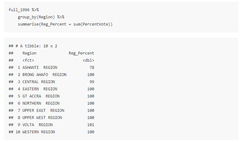
full_1996 <- read_csv("presidential_results_1996.csv")

# Sum of values grouped by Region
full_1996 %>%
  group_by(Region) %>%
  summarise(Regional_Percent = sum(PercentVote))
## # A tibble: 10 x 2
## Region Regional_Percent
## <chr> <dbl>
## 1 ASHANTI REGION 78
## 2 BRONG AHAFO REGION 100
## 3 CENTRAL REGION 99
## 4 EASTERN REGION 100
## 5 GT ACCRA REGION 100
## 6 NORTHERN REGION 100
## 7 UPPER EAST REGION 100
## 8 UPPER WEST REGION 100
## 9 VOLTA REGION 101
## 10 WESTERN REGION 100full_1996$PercentVote <- percent_parties$PercentVote
# save the new data as a .csv file
write.csv(full_1996, "final_presidential_results_1996.csv")
full_1996 %>%
group_by(Region) %>%
summarise(Regional_Percent = sum(PercentVote))## # A tibble: 10 x 2
## Region Regional_Percent
## <chr> <dbl>
## 1 ASHANTI REGION 99.1
## 2 BRONG AHAFO REGION 98.5
## 3 CENTRAL REGION 97.8
## 4 EASTERN REGION 99.7
## 5 GT ACCRA REGION 99.4
## 6 NORTHERN REGION 97.1
## 7 UPPER EAST REGION 93.7
## 8 UPPER WEST REGION 94.8
## 9 VOLTA REGION 99.5
## 10 WESTERN REGION 98.3This has been a very long blog post on an update of a single column. I could have easily updated the values and put a one-liner in Episode 2 informing everyone about the change.
But I wanted to go through the whole process with you and I am glad I did. The presidential results for 1996 Ghanaian elections is available here. So until the next blog post, thank you and bye bye.
